The Imperial High Modernist Cathedral vs The Bazaar

Or: I Thought I was a Programmer but now I’m worried I’m a High Modernist.

Seeing like a State by James C. Scott is a rallying cry against imperialist high modernism. Imperialist high modernism, in the language of the book, is the thesis that:

Big projects are better,
organized big is the only good big,
formal scientific organization is the only good system, and
it is the duty of elites leading the state to make these projects happen — by force if needed

The thesis sounds vague, but it’s really just big. Scott walks through historical examples to flesh out his thesis:

scientific forestry in emerging-scientific Europe
land reforms / standardization in Europe and beyond
the communist revolution in Russia
agricultural reforms in the USSR and Tanzania
modernist city planning in Paris, Brazil, and India

The conclusion, gruesomely paraphrased, is that “top-down, state-mandated reforms are almost never a win for the average subject/victim of those plans ”, for two reasons:

Top-down “reforms” are usually aimed not at optimizing overall resource production, but at optimizing resource extraction by the state.

Example: State-imposed agricultural reforms rarely actually produced more food than peasant agriculture, but they invariably produced more easily countable and taxable food

Top-down order, when it is aimed at improving lives, often misfires by ignoring hyper-local expertise in favor of expansive, dry-labbed formulae and (importantly) academic aesthetics

Example: Rectangular-gridded, mono-cropped, giant farms work in certain Northern European climates, but failed miserably when imposed in tropical climates

Example: Modernist city planning optimized for straight lines, organized districts, and giant apartment complexes to maximize factory production, but at the cost of cities people could actually live in.

However.

Scott, while discussing how Imperial High Modernism has wrought oppression and starvation upon the pre-modern and developing worlds, neglected (in a forgivable oversight), to discuss how first-world Software Engineers have also suffered at the hands of imperial high modernism.

Which is a shame, because the themes in this book align with the most vicious battles fought by corporate software engineering teams. Let this be the missing chapter.

The Imperial High Modernist Cathedral vs The Bazaar

Imperial high modernist urban design optimizes for top-down order and symmetry. High modernist planners had great trust in the aesthetics of design, believing earnestly that optimal function flows from beautiful form.

Or, simpler: “A well-designed city looks beautiful on a blueprint. If it’s ugly from a birds-eye view, it’s a bad city.”

The hallmarks of high modernist urban planning were clean lines, clean distinctions between functions, and giant identical (repeating) structures. Spheres of life were cleanly divided — industry goes here, commerce goes here, houses go here. If this reminds you of autism-spectrum children sorting M&Ms by color before eating them, you get the idea.

Le Corbusier is the face of high modernist architecture, and SlaS focuses on his contributions (so to speak) to the field. While Le Corbusier actualized very few real-world planned cities, he drew a lot of pictures, so we can see his visions of a perfect city:

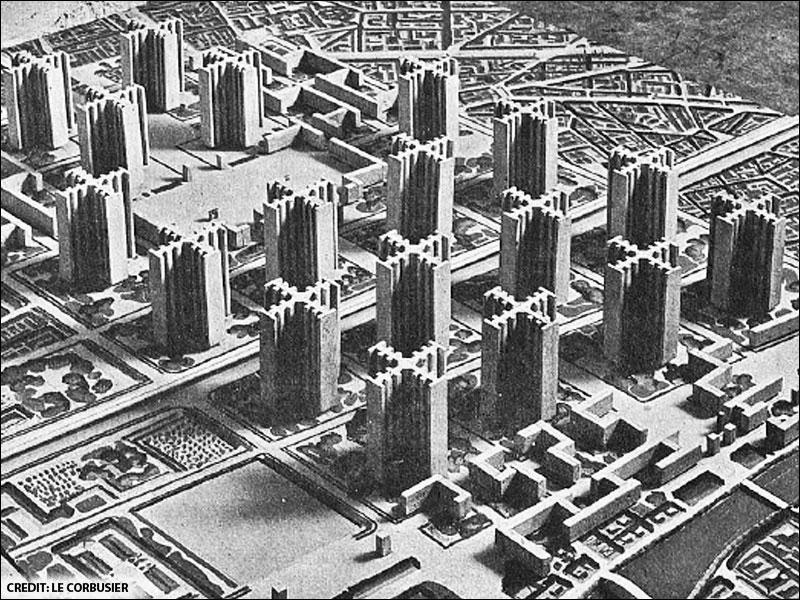
True to form, the cities were beautiful from the air, or perhaps from spectacularly high vantage points — the cities were designed for blueprints, and state legibility. Wide, open roads, straight lines, and everything in an expected place. Shopping malls in one district, not mixed alongside residences. Vast apartment blocks, with vast open plazas between.

Long story short, these cookie-cutter designs were great for urban planners, and convenient for governments. But they were awful for people.

The reshuffling of populations from living neighborhoods into apartment blocks destroyed social structures
Small neighborhood enterprises — corner stores and cafes — had no place in these grand designs. The “future” was to be grand enterprises, in grand shopping districts.
Individuals had no ownership of the city they lived in. There were no neighborhood committees, no informal social bonds.

Fundamentally, the “city from on high” imposed an order upon how people were supposed to live their lives, not even bothering to first learn how the “masses” were already living; he swept clean the structures, habits and other social lube that made the “old” city tick.

In the end, the high modernist cities failed, and modern city planning makes an earnest effort to work with the filthy masses, accepting as natural a baseline of disorder and chaos, to help build a city people want to live in.

If this conclusion makes you twitch, you may be a Software Engineer. Because the same aesthetic preferences which ground Le Corbusier’s gears also are the foundation of “good” software architecture; namely:

Good code is pretty code
Good architecture diagrams visually appear organized

Software devs don’t draft cityscapes, but they do draw Lucidchart wireframes. And a “good” service architecture for a web service would look something like this:

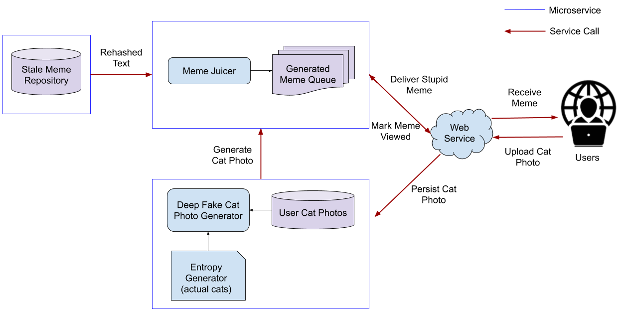
We could try to objectively measure the “good” parts of the architecture:

Each service has only a couple clearly defined inputs and outputs
Data flow is (primarily) unidirectional
Each service appears to do “one logical thing”

But software engineers don’t use a checklist to generate first impressions. Often before even reading the lines, the impression of a good design is,

Yeah, that looks like a decent clean, organized, architecture

In contrast, a “messy” architecture… looks like a mess:

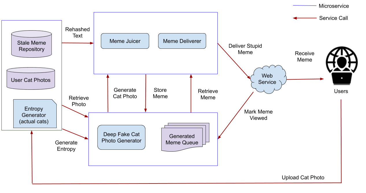
We could likewise break down why it’s a mess:

Services don’t have clearly defined roles
The architecture isn’t layered (the user interacts with backend services?)
There are a lot more service calls
Data flow is not unidirectional

But most software architects wouldn’t wade through the details on first glance. The first reaction is:

Why are there f******* lines everywhere??? What do these microservices even do? How does a user even… I don’t care, burn it.

In practice, most good engineers are ruthless high modernist fascists. Unlike the proto-statist but good-hearted urban planners of the early 1900s (“workers are dumb meat and need to be corralled like cattle, but I want them to be happy cows!”), we wrench the means of production from our code with blood and iron. Inasmuch as the subjects are electrons, this isn’t a failing of the system — it’s the system delivering.

Where this aesthetic breaks down is when these engineers have to coordinate with other human beings — beings who don’t always share the same vision of a system’s platonic ideals. To a perfectionist architect, outside contributions risk tainting the geometric precision with which a system was crafted.

Eric S Raymond famously summarized the two models for building collaborative software in his essay (and later, book): The Cathedral and the Bazaar

Unlike in urban planning, the software Cathedral came first. Every man dies alone, and every programmer codes solo. Corporate, commercial cathedrals were run by a lone (or small team) of ruthless God Emperors, carefully vetting contributions for coherence to a grander plan. The essay summaries the distinctions better than I can rehash, so I’ll quote in length.

The Cathedral model represents mind-made-matter diktat from above:

I believed that the most important software (operating systems and really large tools like Emacs) needed to be built like cathedrals, carefully crafted by individual wizards or small bands of mages working in splendid isolation, with no beta to be released before its time.

The grand exception to this pattern was an upstart open-source Operating System you may have heard of — Linux. Linux took a different approach to design, welcoming with open arms external contributions and all the chaos and dissent they brought:

Linus Torvalds’s style of development – release early and often, delegate everything you can, be open to the point of promiscuity – came as a surprise. No quiet, reverent cathedral-building here – rather, the Linux community seemed to resemble a great babbling bazaar of differing agendas and approaches (aptly symbolized by the Linux archive sites, who’d take submissions from anyone) out of which a coherent and stable system could seemingly emerge only by a succession of miracles.

Eric predicted that the challenges of working within the chaos of the Bazaar — the struggle of herding argumentative usenet-connected cats in a common direction — would be vastly outweighed by the individual skills, experience, and contributions of those cats:

I think the future of open-source software will increasingly belong to people who know how to play Linus’ game, people who leave behind the cathedral and embrace the bazaar. This is not to say that individual vision and brilliance will no longer matter; rather, I think that the cutting edge of open-source software will belong to people who start from individual vision and brilliance, then amplify it through the effective construction of voluntary communities of interest.

Eric was right — Linux dominated, and the Bazaar won. In the open-source world, it won so conclusively that we pretty much just speak the language of the bazaar:

“Community contributions” are the defining measure of health for an Open Source project. No contributions implies a dead project.
“Pull Requests” are how outsiders contribute to OSS projects. Public-editable project wikis are totally standard documentation. Debate (usually) happens on public mailing lists, public Slacks, public Discord servers. Radical transparency is the default.

I won’t take this too far — most successful open-source projects remain a labor of love by a core cadre of believers. But very few successful OSS projects reject outside efforts to flesh out the core vision, be it through documentation, code, or self-machochistic user testing.

The ultimate victory of the Bazaar over the Cathedral mirrors the abandonment of high modernist urban planning. But here it was a silent victory; the difference between cities and software, is that dying software quietly fades away, while dying cities end up on the evening news and on UNICEF donation mailers. The OSS Bazaar won, but the Cathedral faded away without a bang.

Take that, Le Corbusier!

High Modernist Corporate IT vs Developer Metis

At risk of appropriating the suffering of Soviet peasants, there’s another domain where the impositions of high modernism parallel closely with the world of software — in the mechanics of software development.

First, a definition: Metis is a critical but fuzzy concept in SlaS, so I’ll attempt to define it here. Metis is the on-the-ground, hard-to-codify, adaptive knowledge workers use to “get stuff done”. In context of farming, it’s:

“I have 30 variants of rice, but I’ll plant the ones suited to a particular amount of rainfall in a particular year in this particular soil, otherwise the rice will die and everyone will starve to death”

Or in the context of a factory, it’s,

“Sure, that machine works, but when it’s raining and the humidity is high, turning it on will short-circuit, arc through your brain, and turn the operator into pulpy organic fertilizer.”

and so forth.

In the context of programming, metis is the tips and tricks that turn a mediocre new graduate into a great (dare I say, 10x) developer. Using ZSH to get git color annotation. Knowing that, “yeah Lambda is generally cool and great best practice, but since the service is connected to a VPC fat layers, the bursty traffic is going to lead to horrible cold-start times, customers abandoning you, the company going bankrupt, Sales execs forced to live on the streets catching rats and eating them raw.” Etc.

Trusting developer metis means trusting developers to know which tools and technologies to use. Not viewing developers as sources of execution independent of the expertise and tools which turned them into good developers.

Corporate IT — especially at large companies— has an infamous fetish for standardization. Prototypical “standardizations” could mean funneling every dev in an organization onto:

the same hardware, running the same OS (“2015 Macbook Airs for everyone”)
the same IDE (“This is a Visual Studio shop”)
an org-wide standard development methodology (“All changes via GitHub PRs, all teams use 2-week scrum sprints”)
org-wide tool choices (“every team will use Terraform V 0.11.0, on AWS”)

If top-down dev tool standardization reminds you of the Holodomor, the Soviet sorta-genocide side-effect of dekulakizatizing Ukraine, then we’re on the same page.

To be fair, these standardizations are, in the better cases, more defensible than the Soviet agricultural reforms in SlaS. The decisions were (almost always) made by real developers elevated to the role of architect. And not just developers, but really good devs. This is an improvement over the Soviet Union, where Stalin promoted his dog’s favorite groomer to be your district agricultural officer and he knows as much about farming as the average farmer knows about vegan dog shampoo.

But even good standards are sticky, and sticky standards leave a dev team trapped in amber. Recruiting into a hyper-standardized org asymptotically approaches “take and hire the best, and boil them down to high-IQ, Ivy+ League developer paste; apply liberally to under-staffed new initiatives”

When tech startups win against these incumbents, it’s by staying nimble in changing times — changing markets, changing technologies, changing consumer preferences.

To phrase “startups vs the enterprise” in the language of Seeing Like a State: nimble teams — especially nimble engineering teams — can take advantage of metis developer talent to quickly reposition under changing circumstances, while high modernist companies (let’s pick on IBM), like a Soviet collectivist farm, choose to excel at producing standardized money-printing mainframe servers — but only until the weather changes, and the market shifts to the cloud.

Overall

The main thing I struggled with while reading Seeing like a State is that it’s a book about history. The oppression and policy failures are real, but real in a world distant in both space and time — I could connect more more concretely to a discussion of crypto-currency, contemporary public education, or the FDA. Framing software engineering in the language of high modernism helped me ground this book in the world I live in.

Takeaways for my own life? Besides the concrete (don’t collectivize Russian peasant farms, avoid monoculture agriculture at all costs) it will be to view aesthetic simplicity with a skeptical eye. Aesthetic beauty is a great heuristic which guides us towards scalable designs — until it doesn’t.

And when it doesn’t, a bunch of Russian peasants starve to death.

QGIS scripting — Checking point membership within vector layer features

Hit another QGIS snag. This one took a day or so to sort through, and I actually had to write code. So I figured I’d write it up.

I struggled to solve the following problem using QGIS GUI tools:

I have a bunch of points (as a vector layer)
I have a bunch of vector layers of polygons
I want to know, for each point, which layers have at least one feature which contain this point

Speaking more concretely: I have cities (yellow), and I have areas (pink). I want to find which cities are in the areas, and which are not:

I assumed this would be a simple exercise using the GUI tools. It might be. But I could not figure it out. The internet suggests doing a vector layer join, but for whatever reason, joining a point layer to a vector layer crashed QGIS (plus, this is slow overkill for what I need — simple overlap, not full attribute joins).

Luckily, QGIS has rich support for scripting tools. There’s a pretty good tutorial for one example here. The full API is documented using Doxygen here. So I wrote a script to do this. I put the full script on GitHub —you can find it here.

I will preface this before I walk through the code — this is not a clever script. It’s actually really, really dumb, and really, really slow. But I only need this to work once, so I’m not going to implement any potential optimizations (which I’ll describe at the end).

First, the basic-basics: navigate Processing → Toolbox. Click “Create New Script from Template”

This creates — as you might expect — a new script from a template. I’ll go over the interesting bits here, since I had to piece together how to use the API as I went. Glossing over the boilerplate about naming, we only want two parameters: the vector layer with the XY points, and the output layer:

    def initAlgorithm(self, config=None):

        self.addParameter(
            QgsProcessingParameterFeatureSource(
                self.POINT_INPUT,
                self.tr('Input point layer'),
                [QgsProcessing.TypeVectorPoint]
            )
        )

        self.addParameter(
            QgsProcessingParameterFeatureSink(
                self.OUTPUT,
                self.tr('Output layer')
            )
        )

Getting down into the processAlgorithm block, we want to turn this input parameter into a source. We can do that with the built-in parameter methods:

        point_source = self.parameterAsSource(
            parameters,
            self.POINT_INPUT,
            context
        )

        if point_source is None:
            raise QgsProcessingException(self.invalidSourceError(parameters, self.POINT_INPUT))

A more production-ized version of this script would take a list of source layers to check. I could not be bothered to implement that, so I’m just looking at all of them (except the point layer). If it’s a vector layer, we’re checking it:

        vector_layers = []
        
        for key,layer in QgsProject.instance().mapLayers().items():
            if(layer.__class__.__name__ == 'QgsVectorLayer'):
                if(layer.name() != point_source.sourceName()):
                    vector_layers.append(layer)
                else:
                    feedback.pushInfo('Skipping identity point layer: %s:' %point_source.sourceName())

We want our output layer to have two types of attributes:

The original attributes from the point layer
One column for each other layer, for which we can mark presence with a simple 0/1 value.

        output_fields = QgsFields(point_source.fields())
        
        for layer in vector_layers:
            feedback.pushInfo('layer name: %s:' %layer.name())
            
            field = QgsField(layer.name())
            output_fields.append(field)

Similar to the input, we want to turn the parameter into a sink layer:

        (sink, dest_id) = self.parameterAsSink(
            parameters, 
            self.OUTPUT,
            context,
            output_fields,
            point_source.wkbType(),
            point_source.sourceCrs()
        )

        if sink is None:
            raise QgsProcessingException(self.invalidSinkError(parameters, self.OUTPUT))

Although it seems like a “nice to have”, tracking progress as we iterate through our points is pretty important; this script ran for 24 hours on the data I ran through it. If I had hit the 2 hour mark with no idea of progress — I’d certainly have given up.

Likewise, unless you explicitly interrupt your script when the operation is cancelled, QGIS has no way to stop progress. Having to force-kill QGIS to stop a hanging processing algorithm is super, duper, annoying:

        points = point_source.getFeatures()        
        total = 100.0 / point_source.featureCount() if point_source.featureCount() else 0

        for current, point in enumerate(points):

            if feedback.isCanceled():
                break

            feedback.setProgress(int(current * total))

From here on, we iterate over the target layers, and add to the target attributes if point is present in any feature in the target layer:

            attr_copy = point.attributes().copy()

            for layer in vector_layers: 
            
                features = layer.getFeatures()
                feature_match = False
                geometry = point.geometry()

                for feature in features:
                    
                    if (feature.geometry().contains(geometry)):
                        feature_match = True
                        break
                    
                if(feature_match):
                    attr_copy.append(1)
                else:
                    attr_copy.append(0)

Last but not least, we just output the feature we’ve put together into the output sink:

            output_feature = QgsFeature(point)
            output_feature.setAttributes(attr_copy)
            feedback.pushInfo('Point attributes: %s' % output_feature.attributes())
            sink.addFeature(output_feature, QgsFeatureSink.FastInsert)

And that’s about it (minus some boilerplate). Click the nifty “Run” button on your script:

Because we wrote this as a QGIS script, we get a nice UI out of it:

When we run this, it creates a new temporary output layer. When we open up the output layer attribute table, we get exactly what we wanted: for each record, a column with a 0/1 for the presence or absence within a given vector layer:

Perfect.

Now, this script is super slow, but we could fix that. Say we have n input points and m total vector features. The obvious fix is to run in better than n*m time — we’re currently checking every point against every feature in every layer. We could optimize this by geo-bucketing the vector layer features:

Break the map into a 10×10 (or whatever) grid
For each vector layer feature, insert the feature into the grid elements it overlaps.
When we check each point for layer membership, only check the features in the grid element it belongs to.

If we’re using k buckets (100, for a 10×10 grid), this takes the cost down to, roughly, k*m + n*m/k, assuming very few features end up in multiple buckets. We spend k*m to assign each feature to the relevant bucket, and then each point only compares against 1/k of the vector features we did before.

I’m not implementing this right now, because I don’t need to, but given the APIs available here, I actually don’t think it would be more than an hour or two of work. I’ll leave it as an exercise to the reader.

Anyway, I’d been doing my best to avoid QGIS scripting, because it seemed a bit hardcore for a casual like me. Turned out to be pretty straightforward, so I’ll be less of a wimp in the future. I’ll follow up soon™ with what I actually used this script for.

Using TravisCI to deploy to Maven Central via Git tagging (aka death to commit clutter)

jbool_expressions is a small OSS library I maintain. To make it easy to use, artifacts are published to Maven Central. I have never been happy with my process for releasing to Maven Central; the releases were done manually (no CI) on my laptop and felt fragile.

I wanted to streamline this process to meet a few requirements:

All deployments should happen from a CI system; nothing depends on laptop state (I don’t want to lose my encryption key when I get a new laptop)
Every commit to master should automatically publish a SNAPSHOT artifact to Sonatype (no manual snapshot release process)
Cutting a proper release to Maven Central, when needed, should be straightforward and hard to mess up
Performing releases should not generate commit clutter. Namely, no more of this:

Luckily for me, we recently set up a very similar process for our OSS projects at LiveRamp. I don’t want to claim I figured this all out myself — others at LiveRamp (namely, Josh Kwan) were heavily involved in setting up the encryption parts for the LiveRamp OSS projects which I used as a model.

There’s a lot of information out there about Maven deploys, but I had trouble finding a simple guide which ties it all together in a painless way, so I decided to write it up here.

tl,dr: through some TravisCI and Maven magic, jbool_expressions now publishes SNAPSHOT artifacts to Sonatype on each master commit, and I can now deploy a release to Maven Central with these commands:

$ git tag 1.23
$ git push origin 1.23

To update and publish the next SNAPSHOT version, I can just change and push the version:

$ mvn versions:set -DnewVersion=1.24-SNAPSHOT
$ git commit -am "Update to version 1.24-SNAPSHOT"
$ git push origin master

At no point is anything auto-committed by Maven; the only commits in the Git history are ones I did manually. Obviously I could script these last few steps, but I like that these are all primitive commands, with no magic scripts which could go stale or break halfway through.

The thousand-foot view of the CI build I set up for jbool_expressions looks like this:

jbool_expressions uses TravisCI to run tests and deploys on every commit to master
Snapshots deploy to Sonatype; releases deploy to Maven Central (via a Sonatype staging repository)
Tagged commits publish with a version corresponding to the git tag, by using the versions-maven-plugin mid-build.

The rest of this post walks through the setup necessary to get this all working, and points out the important files (if you’d rather just look around, you can just check out the repository itself)

Set up a Sonatype account

Sonatype generously provides OSS projects free artifact hosting and mirroring to Maven Central. To set up an account with Sonatype OSS hosting, follow the guide here. After creating the JIRA account for issues.sonatype.org, hold onto the credentials — we’ll use to use those later to publish artifacts.

Creating a “New Project” ticket and getting it approved isn’t an instant process; the approval is manual, because Maven Central requires artifact coordinates to reflect actual domain control. Since I wanted to publish my artifacts under the com.bpodgursky coordinates, I needed to prove ownership of bpodgursky.com.

Once a project is approved, we have permission to deploy artifacts two important places:

https://oss.sonatype.org/content/repositories/snapshots, which lets us publish snapshot artifacts
https://oss.sonatype.org/service/local/staging/deploy/maven2/, which lets us deploy artifacts we can promote to Maven Central.

We’ll use both of these later.

Set up TravisCI for your GitHub project.

TravisCI is easy to set up. Follow the documentation here.

Configure Maven + Travis to publish to central

Once we have our Sonatype and Travis accounts enabled, we need to configure a few files to get ourselves publishing to central:

pom.xml
.travis/maven-settings.xml
.travis.yml
.travis/gpg.asc.enc
deploy

I’ll walk through the interesting parts of each.

pom.xml

Most of the interesting publishing configuration happens in the “publish” profile here. The three maven plugins — maven-javadoc-plugin, maven-source-plugin, and maven-gpg-plugin — are all standard and generate artifacts necessary for a central deploy (the gpg plugin requires some configuration we’ll do later). The last one — nexus-staging-maven-plugin — is a replacement for the maven-deploy-plugin, and tells Maven to deploy artifacts through Sonatype.

<distributionManagement>
  <snapshotRepository>
    <id>ossrh</id>
    <url>https://oss.sonatype.org/content/repositories/snapshots</url>
  </snapshotRepository>
  <repository>
    <id>ossrh</id>
    <url>https://oss.sonatype.org/service/local/staging/deploy/maven2/</url>
  </repository>
</distributionManagement>

Fairly straightforward — we want to publish release artifacts to Maven central, but SNAPSHOT artifacts to Sonatype (Maven central doesn’t accept SNAPSHOTs)

.travis/maven-settings.xml

The maven-settings here are configurations to be used during deploys, and inject credentials and buildserver specific configurations:

<servers>
  <server>
    <id>ossrh</id>
    <username>${env.OSSRH_USERNAME}</username>
    <password>${env.OSSRH_PASSWORD}</password>
  </server>
</servers>

The Maven server configurations let us tell Maven how to log into Sonatype so we can deploy artifacts. Later I’ll explain how we get these variables into the build.

<profiles>
  <profile>
    <id>ossrh</id>
    <activation>
      <activeByDefault>true</activeByDefault>
    </activation>
    <properties>
      <gpg.executable>gpg</gpg.executable>
      <gpg.keyname>${env.GPG_KEY_NAME}</gpg.keyname>
      <gpg.passphrase>${env.GPG_PASSPHRASE}</gpg.passphrase>
    </properties>
  </profile>
</profiles>

The maven-gpg-plugin we configured earlier earlier has a number of user properties which need to be configured. Here’s where we set them.

.travis.yml

.travis.yml completely defines how and when TravisCI builds a project. I’ll walk through what we do in this one.

language: java
jdk:
- openjdk10

The header of .travis.yml configures a straightforward Java 10 build. Note, we can (and do) still build at a Java 8 language level, we just don’t want to use a deprecated JDK.

install: "/bin/true"
script:
- "./test"

Maven installs the dependencies it needs during building, so we can just disable the “install” phase entirely. The test script can be inlined if you prefer; it runs a very simple suite:

mvn clean install -q -B

(by running through the “install” phase instead of just “test”, we also catch the “integration-test” and “verify” Maven phases, which are nice things to run in a PR, if they exist).

env:
  global:
  - secure: ...
  - secure: ...
  - secure: ...
  - secure: ...

The next four encrypted secrets were all added via travis. For more details on how TravisCI handles encrypted secrets, see this article. Here, these hold four variables we’ll use in the deploy script:

travis encrypt OSSRH_PASSWORD='<sonatype password>' --add env.global
travis encrypt OSSRH_USERNAME='<sonatype username>' --add env.global
travis encrypt GPG_KEY_NAME='<gpg key name>' --add env.global
travis encrypt GPG_PASSPHRASE='<pass>' --add env.global

The first two variables are the Sonatype credentials we created earlier; these are used to authenticate to Sonatype to publish snapshots and release artifacts to central. The last two are for the GPG key we’ll be using to sign the artifacts we publish to Maven central. Setting up GPG keys and using them to sign artifacts is outside the scope of this post; Sonatype has documented how to set up your GPG key here, and how to use it to sign your Maven artifacts here.

Next we need to set up our GPG key. To sign our artifacts in a Travis build, we need the GPG key available. Again, set this up by having Travis encrypt the entire file:

travis encrypt-file .travis/gpg.asc --add

In this case, gpg.asc is the gpg key you want to use to sign artifacts. This will create .travis/gpg.asc.enc — commit this file, but do not commit gpg.asc.

Travis will have added a block to .travis.yml that looks something like this:

before_deploy:
- openssl aes-256-cbc -K $encrypted_f094dd62560a_key -iv $encrypted_f094dd62560a_iv -in .travis/gpg.asc.enc -out .travis/gpg.asc -d

Travis defaults to “before_install”, but in this case we don’t need gpg.asc available until the artifact is deployed.

deploy:
-
  skip_cleanup: true
  provider: script
  script: ./deploy
  on:
    branch: master
-
  skip_cleanup: true
  provider: script
  script: ./deploy
  on:
    tags: true

Here we actually set up the artifact to deploy (the whole point of this exercise). We tell Travis to deploy the artifact under two circumstances: first, for any commit to master; second, if there were tags pushed. We’ll use the distinction between the two later.

deploy

The deploy script handles the actual deployment. After a bit of input validation, we get to the important parts:

gpg --fast-import .travis/gpg.asc

This imports the gpg key we decrypted earlier — we need to use this to sign artifacts.

if [ ! -z "$TRAVIS_TAG" ]
then
    echo "on a tag -> set pom.xml <version> to $TRAVIS_TAG"
    mvn --settings "${TRAVIS_BUILD_DIR}/.travis/mvn-settings.xml" org.codehaus.mojo:versions-maven-plugin:2.1:set -DnewVersion=$TRAVIS_TAG 1>/dev/null 2>/dev/null
else
    echo "not on a tag -> keep snapshot version in pom.xml"
fi

This is the important part for eliminating commit clutter. Whenever a tag is pushed — aka, whenever $TRAVIS_TAG exists — we use the versions-maven-plugin to temporarily set the project’s version to that tag. Specifically,

$ git tag 1.23
$ git push origin 1.23

The committed artifact version in pom.xml doesn’t change. It doesn’t matter what the version is in pom.xml in master — we want to publish this version as 1.23.

mvn deploy -P publish -DskipTests=true --settings "${TRAVIS_BUILD_DIR}/.travis/mvn-settings.xml"

Last but not least, the actual deploy. Since we configured our distributionManagement section above with different snapshot and release repositories, we don’t need to think about the version anymore — if it’s still SNAPSHOT (like in the pom), it goes to Sonatype; if we pushed a release tag, it’s headed for central.

That’s it!

Before this setup, I was never really happy with my process for cutting a release and getting artifacts into Maven Central — the auto-generated git commits cluttered the history and it was too easy for a release to fail halfway. With this process, it’s almost impossible for me to mess up a release.

Hopefully this writeup helps a few people skip the trial-and-error part of getting OSS Java artifacts released. Let me know if I missed anything, or there’s a way to make this even simpler.

Migrating LiveRamp’s Hadoop infrastructure to GCP

At Google Next 2019, co-workers Sasha Kipervarg, Patrick Raymond and I presented about how we migrated our company’s on-premise big-data Hadoop environment to GCP, from both a technical and cultural perspective. You can view the presentation and slides on YouTube:

Our Google Next presentation did not give us enough time to go into deep technical details; to give a more in-depth technical view of our migration, I’ve put together a series of blog posts on the LiveRamp engineering blog, with an emphasis on how we migrated our Hadoop environment, the infrastructure my team is responsible for maintaining:

Part 1 where I discuss our Hadoop environment, why we decided to migrate LiveRamp to the cloud, and how we chose GCP.

Part 2 where I discuss the design we chose for our Hadoop environment on GCP.

Part 3 where I discuss the migration process and system architecture which let teams incrementally migrate applications to the cloud.

Part 4 written by coworker Porter Westling, where he discusses how we worked around our data center egress bandwidth restrictions.

Part 5 where I discuss LiveRamp’s use of the cloud going forward, and the cultural changes enabled by migrating to the cloud from an on-premise environment.

LiveRamp’s migration into GCP has been my (and my team’s) primary objective for over a year, and we’ve learned (sometimes painfully) a ton on the way. Hopefully these articles help others who are planning big-data cloud migrations skip a few painful lessons.

Procedural star rendering with three.js and WebGL shaders

Over the past few months I’ve been working on a WebGL visualization of earth’s solar neighborhood — that is, a 3D map of all stars within 75 light years of Earth, rendering stars and (exo)planets as accurately as possible. In the process I’ve had to learn a lot about WebGL (specifically three.js, the WebGL library I’ve used). This post goes into more detail about how I ended up doing procedural star rendering using three.js.

The first iteration of this project rendered stars as large balls, with colors roughly mapped to star temperature. The balls did technically tell you where a star was, but it’s not a particularly compelling visual:

Pretty much any interesting WebGL or OpenGL animation uses vertex and fragment shaders to render complex details on surfaces. In some cases this just means mapping a fixed image onto a shape, but shaders can also be generated randomly, to represent flames, explosions, waves etc. three.js makes it easy to attach custom vertex and fragment shaders to your meshes, so I decided to take a shot at semi-realistic (or at least, cool-looking) star rendering with my own shaders.

Some googling brought me to a very helpful guide on the Seeds of Andromeda dev blog which outlined how to procedurally render stars using OpenGL. This post outlines how I translated a portion of this guide to three.js, along with a few tweaks.

The full code for the fragment and vertex shaders are on GitHub. I have images here, but the visuals are most interesting on the actual tool (http://uncharted.bpodgursky.com/) since they are larger and animated.

Usual disclaimer — I don’t know anything about astronomy, and I’m new to WebGL, so don’t assume that anything here is “correct” or implemented “cleanly”. Feedback and suggestions welcome.

My goal was to render something along the lines of this false-color image of the sun:

In the final shader I implemented:

the star’s temperature is mapped to an RGB color
noise functions try to emulate the real texture
- a base noise function to generate granules
- a targeted negative noise function to generate sunspots
- a broader noise function to generate hotter areas
a separate corona is added to show the star at long distances

Temperature mapping
The color of a star is determined by its temperature, following the black body radiation, color spectrum:

(sourced from wikipedia)

Since we want to render stars at the correct temperature, it makes sense to access this gradient in the shader where we are choosing colors for pixels. Unfortunately, WebGL limits the size of uniforms to a couple hundred on most hardware, making it tough to pack this data into the shader.

In theory WebGL implements vertex texture mapping, which would let the shader fetch the RGB coordinates from a loaded texture, but I wasn’t sure how to do this in WebGL. So instead I broke the black-body radiation color vector into a large, horrifying, stepwise function:

bool rbucket1 = i < 60.0; // 0, 255 in 60 bool rbucket2 = i >= 60.0 && i < 236.0;  //   255,255
…
float r =
float(rbucket1) * (0.0 + i * 4.25) +
float(rbucket2) * (255.0) +
float(rbucket3) * (255.0 + (i - 236.0) * -2.442) +
float(rbucket4) * (128.0 + (i - 288.0) * -0.764) +
float(rbucket5) * (60.0 + (i - 377.0) * -0.4477)+
float(rbucket6) * 0.0;

Pretty disgusting. But it works! The full function is in the shader here

Plugging in the Sun’s temperature (5,778) gives us an exciting shade of off-white:

While beautiful, we can do better.

Base noise function (granules)

Going forward I diverge a bit from the SoA guide. While the SoA guide chooses a temperature and then varies the intensity of the texture based on a noise function, I instead fix high and low surface temperatures for the star, and use the noise function to vary between them. The high and low temperatures are passed into the shader as uniforms:

 var material = new THREE.ShaderMaterial({
   uniforms: {
     time: uniforms.time,
     scale: uniforms.scale,
     highTemp: {type: "f", value: starData.temperatureEstimate.value.quantity},
     lowTemp: {type: "f", value: starData.temperatureEstimate.value.quantity / 4}
   },
   vertexShader: shaders.dynamicVertexShader,
   fragmentShader: shaders.starFragmentShader,
   transparent: false,
   polygonOffset: -.1,
   usePolygonOffset: true
 });

All the noise functions below shift the pixel temperature, which is then mapped to an RGB color.

Convection currents on the surface of the sun generate noisy “granules” of hotter and cooler areas. To represent these granules an available WebGL implementation of 3D simplex noise. The base noise for a pixel is just the simplex noise at the vertex coordinates, plus some magic numbers (simply tuned to whatever looked “realistic”):

void main( void ) {
float noiseBase = (noise(vTexCoord3D , .40, 0.7)+1.0)/2.0;

The number of octaves in the simplex noise determines the “depth” of the noise, as zoom increases. The tradeoff of course is that each octave increases the work the GPU computes each frame, so more octaves == fewer frames per second. Here is the sun rendered at 2 octaves:

4 octaves (which I ended up using):

and 8 octaves (too intense to render real-time with acceptable performance):

Sunspots

Sunspots are areas on the surface of a star with a reduced surface temperature due to magnetic field flux. My implementation of sunspots is pretty simple; I take the same noise function we used for the granules, but with a decreased frequency, higher amplitude and initial offset. By only taking the positive values (the max function), the sunspots show up as discrete features rather than continuous noise. The final value (“ss”) is then subtracted from the initial noise.

float frequency = 0.04;
float t1 = snoise(vTexCoord3D * frequency)*2.7 -  1.9;
float ss = max(0.0, t1);

This adds only a single snoise call per pixel, and looks reasonably good:

Additional temperature variation

To add a bit more noise, the noise function is used one last time, this time to add temperature in broader areas, for a bit more noise:

float brightNoise= snoise(vTexCoord3D * .02)*1.4- .9;
float brightSpot = max(0.0, brightNoise);

float total = noiseBase - ss + brightSpot;

All together, this is what the final shader looks like:

Corona

Stars are very small, on a stellar scale. The main goal of this project is to be able to visually hop around the Earth’s solar neighborhood, so we need to be able to see stars at a long distance (like we can in real life).

The easiest solution is to just have a very large fixed sprite attached at the star’s location. This solution has some issues though:

being inside a large semi-opaque sprite (ex, when zoomed up towards a star) occludes vision of everything else
scaled sprites in Three.js do not play well with raycasting (the raycaster misses the sprite, making it impossible to select stars by mousing over them)
a fixed sprite will not vary its color by star temperature

I ended up implementing a shader which implemented a corona shader with

RGB color based on the star’s temperature (same implementation as above)
color near the focus trending towards pure white
size was proportional to camera distance (up to a max distance)
a bit of lens flare (this didn’t work very well)

Full code here. Lots of magic constants for aesthetics, like before.

Close to the target star, the corona is mostly occluded by the detail mesh:

At a distance the corona remains visible:

On a cooler (temperature) star:

The corona mesh serves two purposes

calculating intersections during raycasting (to enable targeting stars via mouseover and clicking)
star visibility

Using a custom shader to implement both of these use-cases let me cut the number of rendered three.js meshes in half; this is great, because rendering half as many objects means each frame renders twice as quickly.

Conclusions

This shader is a pretty good first step, but I’d like to make a few improvements and additions when I have a chance:

Solar flares (and other 3D surface activity)
More accurate sunspot rendering (the size and frequency aren’t based on any real science)
Fix coronas to more accurately represent a star’s real visual magnitude — the most obvious ones here are the largest ones, not necessarily the brightest ones

My goal is to follow up this post a couple others about parts of this project I think turned out well, starting with the orbit controls (the logic for panning the camera around a fixed point while orbiting).

3D map of Solar Neighborhood using three.js (again!)

A few years ago I posted about a WebGL visualization of the neighborhood around our sun. It was never as polished as I wanted, so on-and-off over the past few months I’ve been working on making it more interesting. The project is still located here:

http://uncharted.bpodgursky.com/

The code is still hosted on GitHub:

https://github.com/bpodgursky/uncharted

Two of the improvements I’m especially excited about. First the star rendering now uses glsl shaders which are based on the star’s temperature, giving cool (and animated!) visuals:

Second, all known exoplanets (planets orbiting stars besides our Sun) are rendered around their parent stars. The textures here are of course fake, but the orbits are accurate where the data is known:

I’ve also included all the full planets in our solar system with full textures and (hopefully accurate) orbits:

I’ve updated the README on the GitHub project with all the changes (I’ve also totally reworked the controls).

I’m going to try to write some more granular posts about what actually went into the three.js and glsl to implement this, since I learned a ton in the process.

Catalog of Life Taxonomic Tree

A small visualization I’ve wanted to do for a while is a tree of life graph — visualizing all known species and their relationships.

Recently I found that the Catalog of Life project has a very accessible database of all known species / taxonomic groups and their relationships, available for download here. This let me put together a simple site backed by their database, available here:

http://taxontree.bpodgursky.com/

All the source code is available on Github.

Design

I’ve used dagre + d3 on a number of other graph visualization projects, so dagre-d3 was the natural choice for the visualization component. The actual code required to do the graph building and rendering is pretty trivial.

The data fetching was a bit trickier. Since pre-loading tens of millions of records was obviously unrealistic, I had to implement a graph class (BackedBiGraph) which lazily expands and collapses, using user-provided callbacks to fetch new data. In this case, the callbacks were just ajax calls back to the server.

The Catalog of Life database did not come with a Java client, so I thought this would be a good opportunity to use jOOQ to generate Java models and query builders corresponding to the COL database, since I am allergic to writing actual SQL queries. This ended up working very well — configuring the jOOQ Maven plugin was simple, and the generated code made writing the queries trivial:

 private Collection&lt;TaxonNodeInfo&gt; taxonInfo(Condition condition) {
return context.select()
.from(TAXON)
.leftOuterJoin(TAXON_NAME_ELEMENT)
.on(TAXON.ID.equal(TAXON_NAME_ELEMENT.TAXON_ID))
.leftOuterJoin(SCIENTIFIC_NAME_ELEMENT)
.on(SCIENTIFIC_NAME_ELEMENT.ID.equal(TAXON_NAME_ELEMENT.SCIENTIFIC_NAME_ELEMENT_ID))
.where(condition).fetch().stream().map(record -&gt; new TaxonNodeInfo(
record.into(TAXON),
record.into(TAXON_NAME_ELEMENT),
record.into(SCIENTIFIC_NAME_ELEMENT)
)).collect(Collectors.toList());
}

All in all, there are a lot of rough edges still, but dagre, d3 and jOOQ made this a much easier project than expected. The code is on Github, so suggestions, improvements, or bugfixes are always welcome.

D3 NLP Visualizer Update

A couple years ago I put together a simple NLP parse tree visualizer demo which used d3 and the dagre layout library. At the time, integrating dagre with d3 required a bit of manual work (or copy-paste); however, since then dagre-d3 library was split out of dagre which added an easy API for adding and removing nodes. Even though the library isn’t under active development, I think it’s still the most powerful pure-JS directed graph layout library out there.

An example from the wiki shows how simple the the dagre-d3 API is for creating directed graphs, abbreviated here:

    // Create the input graph
    var g = new dagreD3.graphlib.Graph()
      .setGraph({})
      .setDefaultEdgeLabel(function() { return {}; });

    // Here we"re setting nodeclass, which is used by our custom drawNodes function
    // below.
    g.setNode(0,  { label: "TOP", class: "type-TOP" });

    // ... snip

    // Set up edges, no special attributes.
    g.setEdge(3, 4);
    
    // ... snip
    // Create the renderer
    var render = new dagreD3.render();

    var svg = d3.select("svg"),
        svgGroup = svg.append("g");

    // Run the renderer. This is what draws the final graph.
    render(d3.select("svg g"), g);

Since that original demo site still gets a fair amount of traffic, I thought it would be good to update it to use dagre-d3 instead of the original hand-rolled bindings (along with other cleanup). You can see the change set required here.

The other goal was to re-familiarize myself with d3 and dagre, since I have a couple projects in mind which would make heavy use of both. Hopefully I’ll have something to post here in the next couple months.

Simple Boolean Expression Manipulation in Java

I’ve worked on a couple projects recently where I needed to be able to do some lightweight propositional expression manipulation in Java. Specifically, I wanted to be able to:

Let a user input simple logical expressions, and parse them into Java data structures
Evaluate the truth of the statement given values for each variable
Incrementally update the expression as values are assigned to the variables
If the statement given some variable assignments is not definitively true or false, show which terms remain.
Perform basic simplification of redundant terms (full satisfiability is of course NP hard, so this would only include basic simplification)

I couldn’t find a Java library which made this particularly easy; a couple stackoverflow questions I found didn’t have any particularly easy solutions. I decided to take a shot at implementing a basic library. The result is on GitHub as the jbool_expressions library.

(most of the rest of this is copied from the README, so feel free to read it there.)

Using the library, a basic propositional expression is built out of the types And, Or, Not, Variable and Literal. All of these extend the base type Expression. An Expression can be built programatically:

    Expression expr = And.of(
        Variable.of("A"),
        Variable.of("B"),
        Or.of(Variable.of("C"), Not.of(Variable.of("C"))));
    System.out.println(expr);

or by parsing a string:

    Expression expr =
        ExprParser.parse("( ( (! C) | C) & A & B)");
    System.out.println(expr);

The expression is the same either way:

    ((!C | C) & A & B)

We can do some basic simplification to eliminate the redundant terms:

    Expression simplified = RuleSet.simplify(expr);
    System.out.println(expr);

to see the redundant terms are simplified to “true”:

    (A & B)

We can assign a value to one of the variables, and see that the expression is simplified after assigning “A” a value:

    Expression halfAssigned = RuleSet.assign(
        simplified,
        Collections.singletonMap("A", true)
    );
    System.out.println(halfAssigned);

We can see the remaining expression:

If we assign a value to the remaining variable, we can see the expression evaluate to a literal:

    Expression resolved = RuleSet.assign(
        halfAssigned,
         Collections.singletonMap("B", true)
     );
    System.out.println(resolved);

    true

All expressions are immutable (we got a new expression back each time we performed an operation), so we can see that the original expression is unmodified:

    System.out.println(expr);

    ((!C | C) & A & B)

Expressions can also be converted to sum-of-products form:

    Expression nonStandard = PrefixParser.parse(
        "(* (+ A B) (+ C D))"
    );

    System.out.println(nonStandard);

    Expression sopForm = RuleSet.toSop(nonStandard);
    System.out.println(sopForm);

    ((A | B) & (C | D))
    ((A & C) | (A & D) | (B & C) | (B & D))

You can build the library yourself or grab it via maven:


<dependency>
    <groupId>com.bpodgursky</groupId>
    <artifactId>jbool_expressions</artifactId>
    <version>1.3</version>
</dependency>

Happy to hear any feedback / bugs / improvements etc. I’d also be interested in hearing how other people have dealt with this problem, and if there are any better libraries out there.

Average Income per Programming Language

Update 8/21: I’ve gotten a lot of feedback about issues with these rankings from comments, and have tried to address some of them here. The data there has been updated to include confidence intervals.

———————————————————————————————————

A few weeks ago I described how I used Git commit metadata plus the Rapleaf API to build aggregate demographic profiles for popular GitHub organizations (blog post here, per-organization data available here).

I was also interested in slicing the data somewhat differently, breaking down demographics per programming language instead of per organization. Stereotypes about developers of various languages abound, but I was curious how these lined up with reality. The easiest place to start was age, income, and gender breakdowns per language. Given the data I’d already collected, this wasn’t too challenging:

For each repository I used GitHub’s estimate of a repostory’s language composition. For example, GitHub estimates this project at 75% Java.
For each language, I aggregated incomes for all developers who have contributed to a project which is at least 50% that language (by the above measure).
I filtered for languages with > 100 available income data points.

Here are the results for income, sorted from lowest average household income to highest:

Language	Average Household Income ($)	Data Points
Puppet	87,589.29	112
Haskell	89,973.82	191
PHP	94,031.19	978
CoffeeScript	94,890.80	435
VimL	94,967.11	532
Shell	96,930.54	979
Lua	96,930.69	101
Erlang	97,306.55	168
Clojure	97,500.00	269
Python	97,578.87	2314
JavaScript	97,598.75	3443
Emacs Lisp	97,774.65	355
C#	97,823.31	665
Ruby	98,238.74	3242
C++	99,147.93	845
CSS	99,881.40	527
Perl	100,295.45	990
C	100,766.51	2120
Go	101,158.01	231
Scala	101,460.91	243
ColdFusion	101,536.70	109
Objective-C	101,801.60	562
Groovy	102,650.86	116
Java	103,179.39	1402
XSLT	106,199.19	123
ActionScript	108,119.47	113

Here’s the same data in chart form:

Most of the language rankings were roughly in line with my expectations, to the extent I had any:

Haskell is a very academic language, and academia is not known for generous salaries
PHP is a very accessible language, and it makes sense that casual / younger / lower paid programmers can easily contribute
On the high end of the spectrum, Java and ActionScript are used heavily in enterprise software, and enterprise software is certainly known to pay well

On the other hand, I’m unfamiliar with some of the other languages on the high/low ends like XSLT, Puppet, and CoffeeScript. Any ideas on why these languages ranked higher or lower than average?

Caveats before making too many conclusions from the data here:

These are all open-source projects, which may not accurately represent compensation among closed-source developers
Rapleaf data does not have total income coverage, and the sample may be biased
I have not corrected for any other skew (age, gender, etc)
I haven’t crawled all repositories on GitHub, so the users for whom I have data may not be a representative sample

That said, even though the absolute numbers may be biased, I think this is a good starting point when comparing relative compensation between languages.

Let me know any thoughts or suggestions about the methodology or the results. I’ll follow up soon with age and gender breakdowns per language in a similar fashion.