I thought was done learning new QGIS tools for a while. Turns out I needed to learn one more trick with QGIS — the Gaussian filter tool. The Gaussian filter is sparsely documented basically undocumented, so I figured I’d write up an post on how I used it to turn a raster image into vector layers of gradient bands.
Motivation: In my spare time I’m adding more layers to the site I’ve been building which maps out disaster risks. California was mostly on fire last year, so I figured wildfires were a pretty hot topic right now.
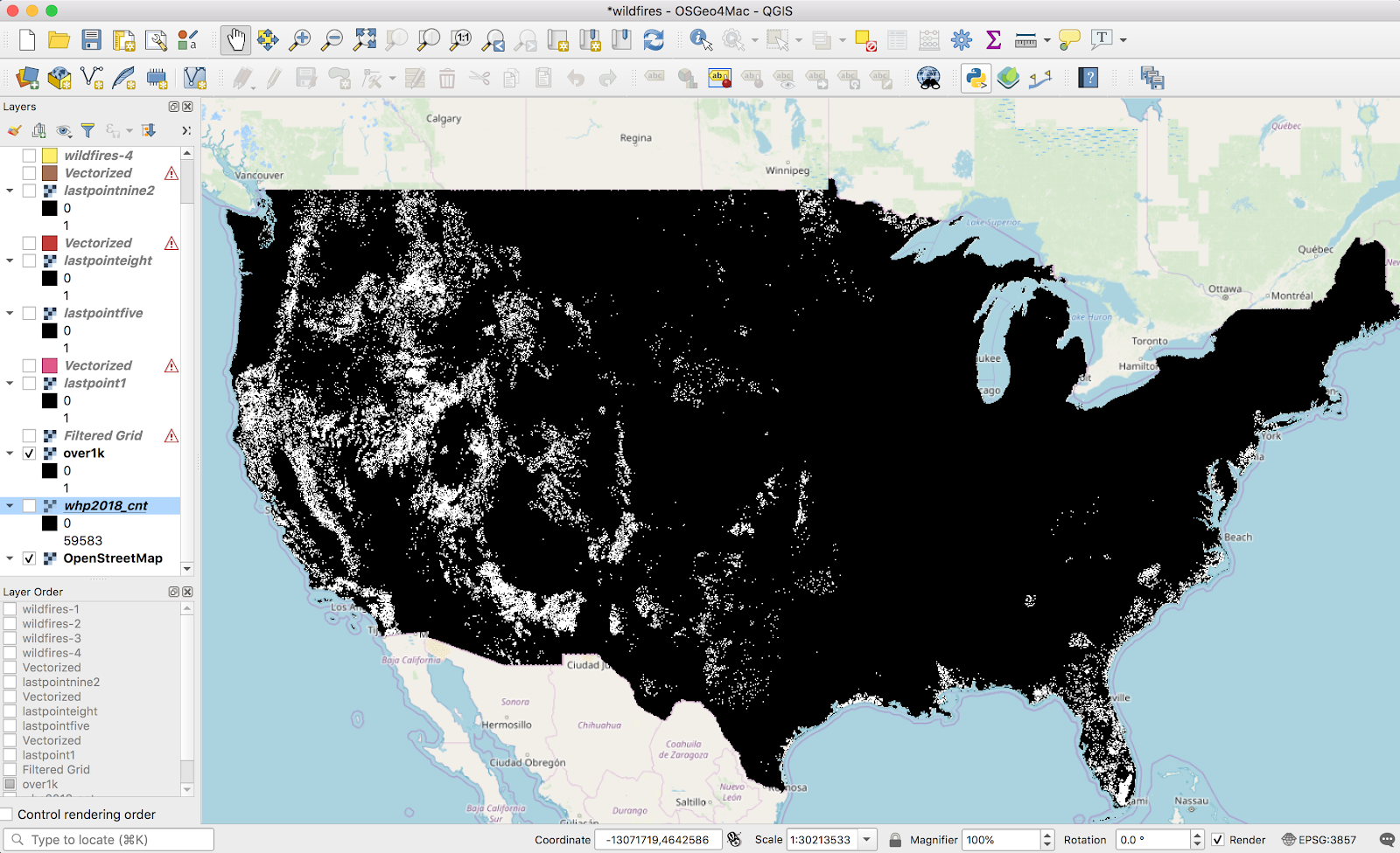
The most useful data-source I found for wildfire risk was this USDA-sourced raster data of overall 2018 wildfire risk, at a pretty fine gradient level. I pulled this into QGIS:
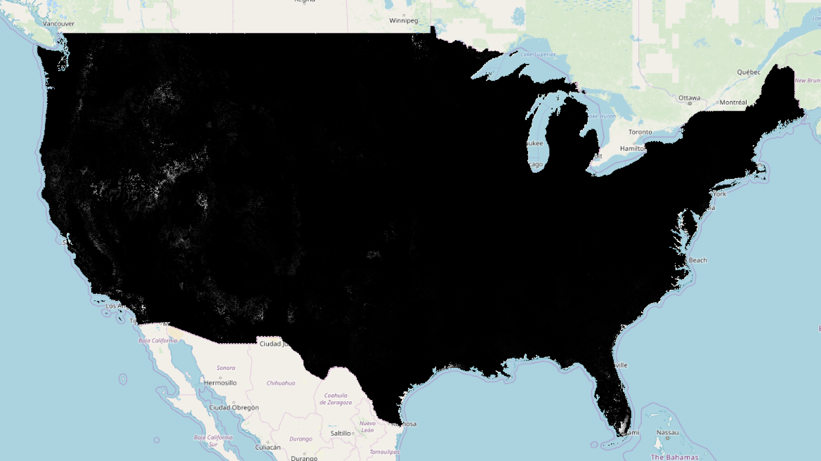
(I’m using the continuous WHP from the site I linked). Just to get a sense of what the data looked like, I did some basic styling to make near-0 values transparent, and map the rest of the values to a familiar color scheme:
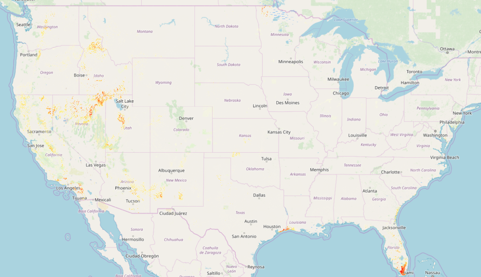
This actually looks pretty good as a high-level view, but the data is actually super grainy when you zoom in (which makes sense — the data was collected to show national maps):
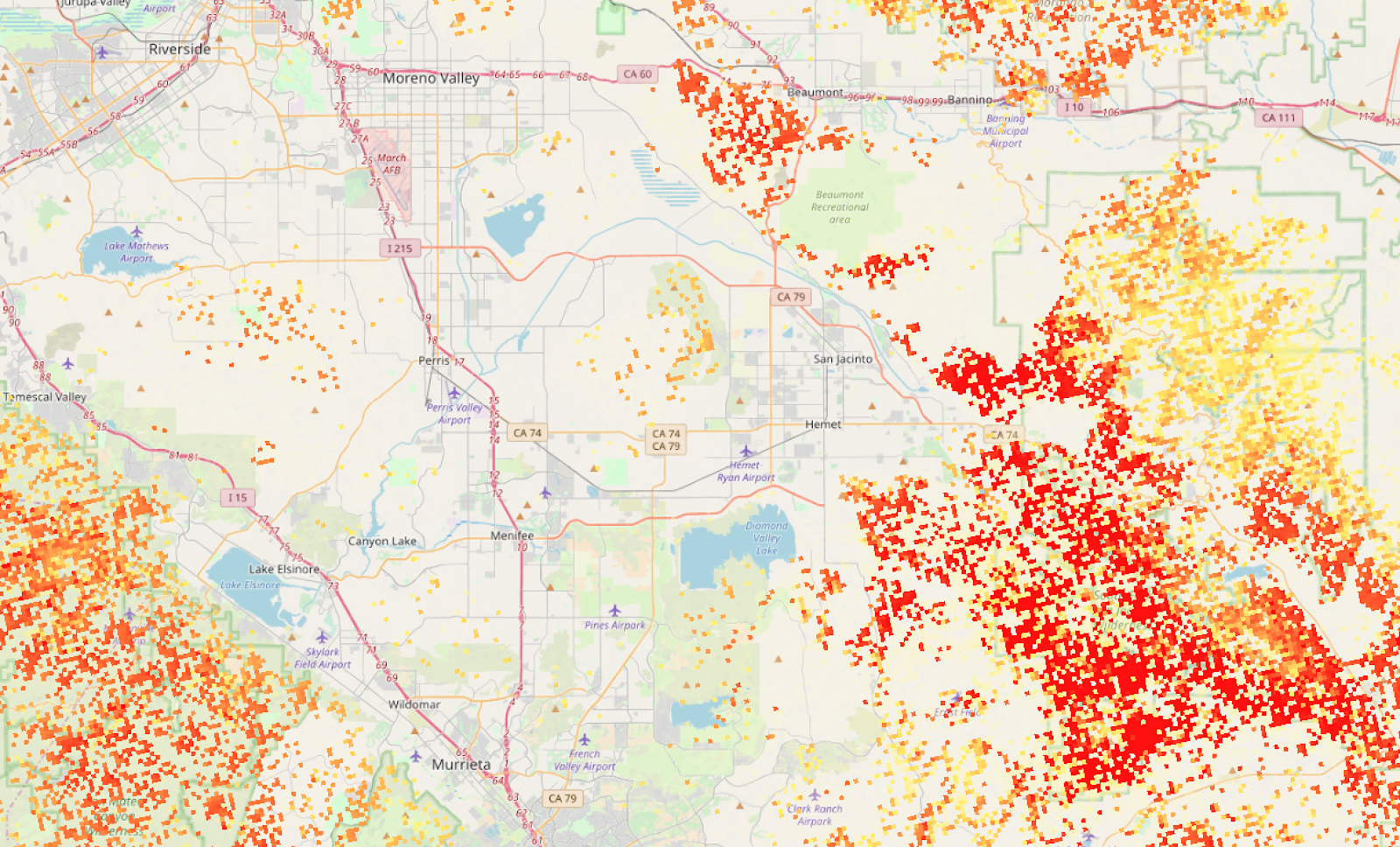
This is a bit grainy to display as-is at high zoom levels. Also, raster data, although very precise is (1) slow to load for large maps and (2) difficult to work with in the browser — in MapBox I’m not able to remap raster values or easily get the value at a point (eg, on mouse click). I wanted this data available as a vector layer, and I was willing to sacrifice a bit of granularity to get there.
The rest of this post will be me getting there. The basic steps will be:
- Filtering out low values from the source dataset
- Using a very slow, wide, Gaussian filter to “smooth” the input raster
- Using the raster calculator to extract discrete bands from the data
- Converting the raster to polygons (“polygonalize”)
- Putting it together and styling it
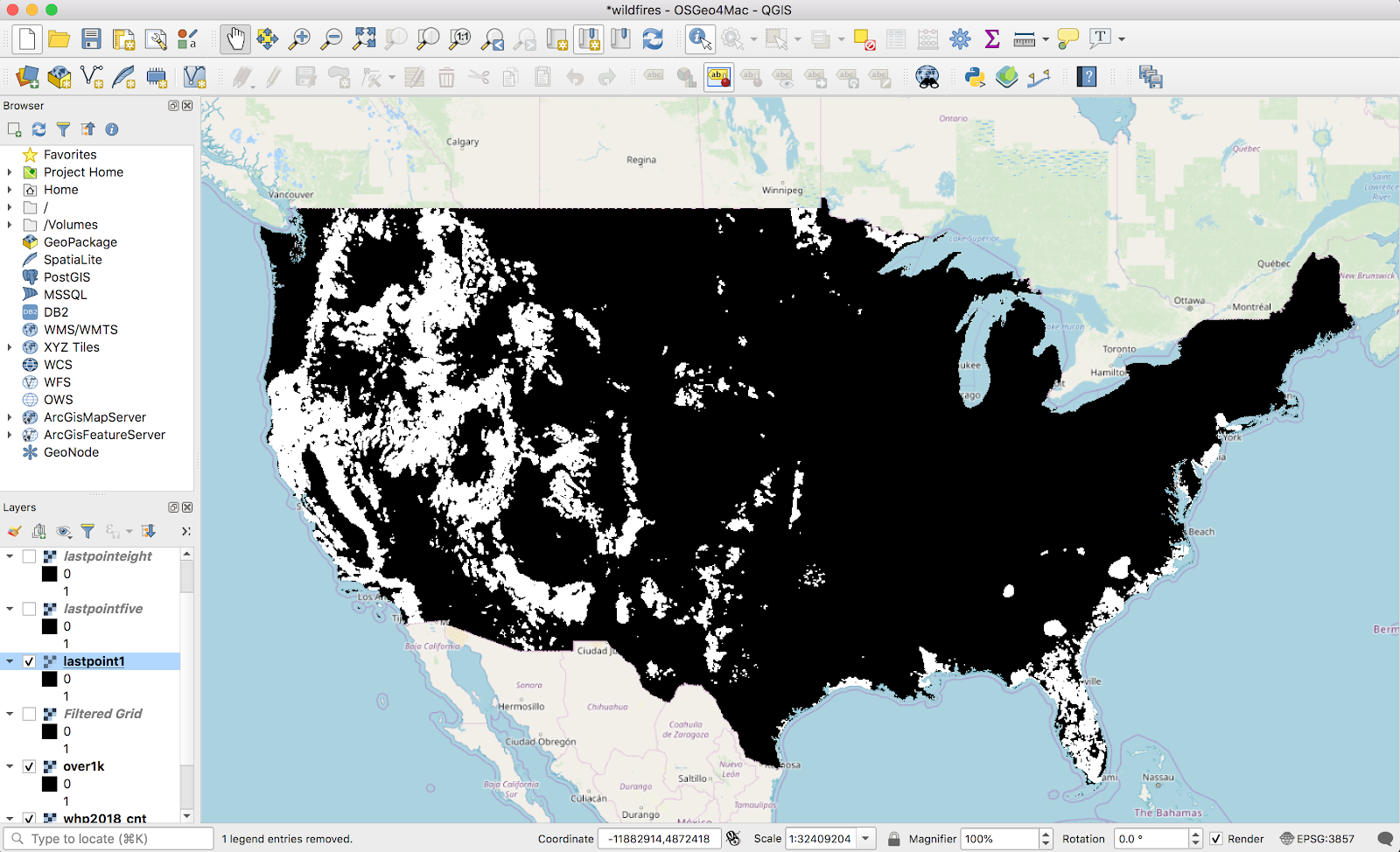
The first thing I did was filter values out of the original raster image below a certain threshold using the raster calculator. The only justification I have for this is “the polygonalization never finished if I didn’t”. Presumably this calculation is only feasible for reasonably-sized raster maps:
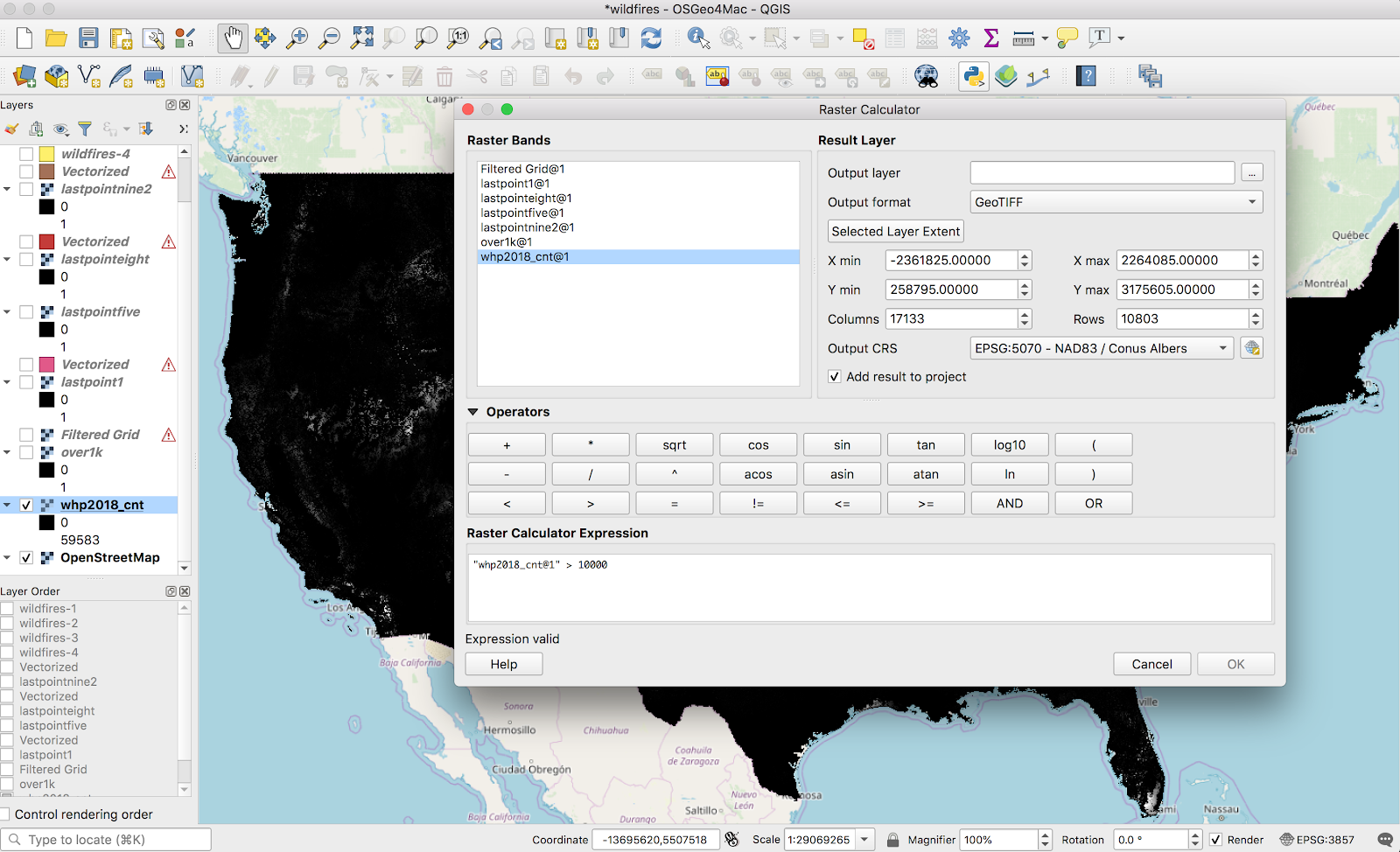
(I iterated on this, so the screenshot is wrong: I used a threshold of 1,000 in the final version). The result looks like this:
Next step is the fancy new tool — the Gaussian filter. A Gaussian filter, or blur, as I’ve seen elsewhere, is kind of a fancy “smudge” tool. It’s available via Processing → Toolbox → SAGA → Raster filter.
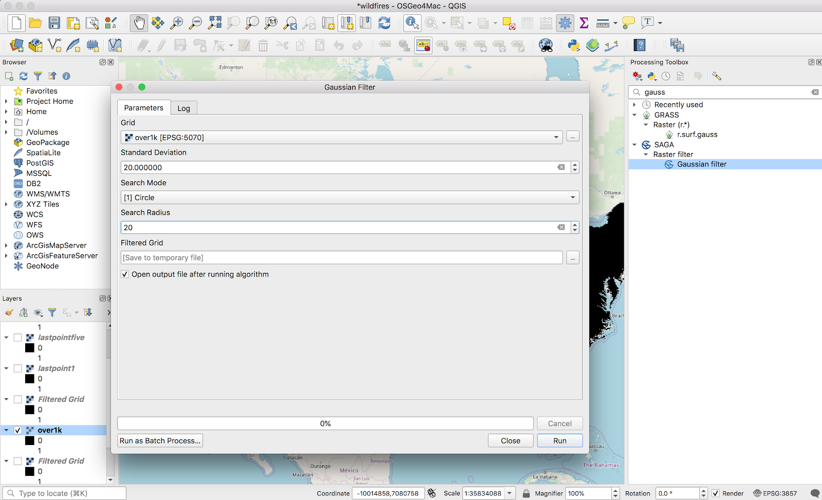
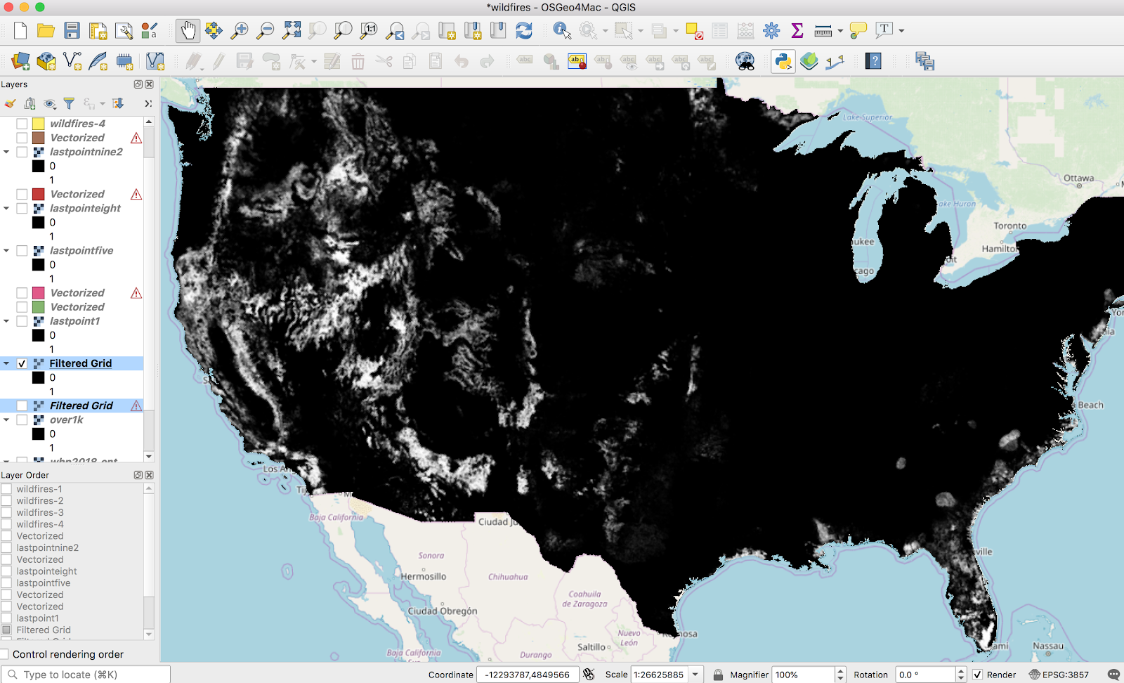
This took forever to run. Naturally, the larger values I used for the radius, the longer it took. Iterated on the numbers here for quite a while, with no real scientific basis; I settled on 20 Standard Deviation and 20 search radius (pixels), because it worked. There is no numerical justification for those numbers. The result looks like this:
Now, we can go back to what I did a few weeks ago — turning a raster into vectors with the raster calculator and polygonalization. I did a raster calculator on this layer (a threshold of .1 here, not shown):
These bands are actually continuous enough that we can vectorize it without my laptop setting any polar bears on fire. I ran through the normal Raster → Conversion → Polygonalize tool to create a new vector layer:
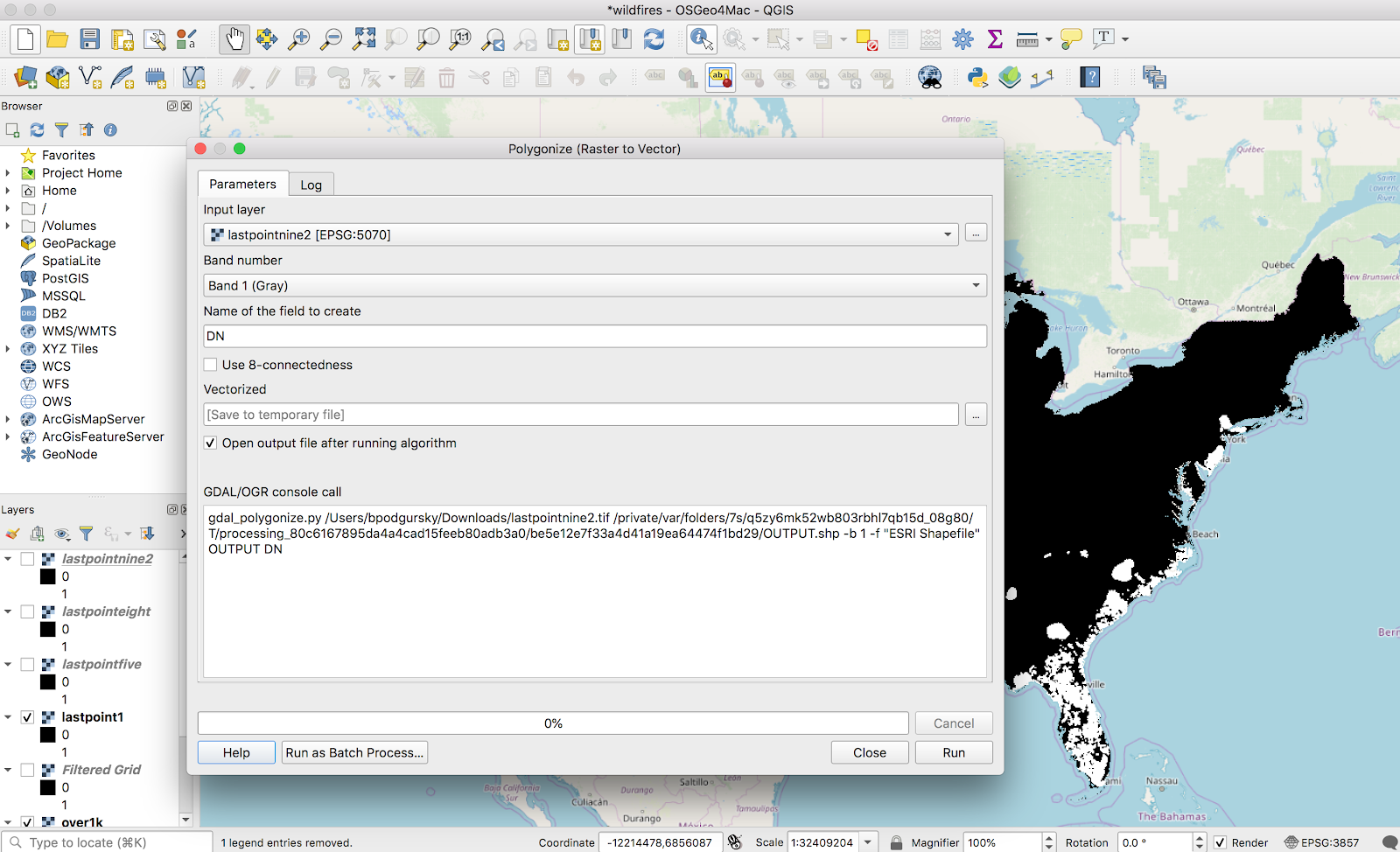
This looks like what we’d expect:
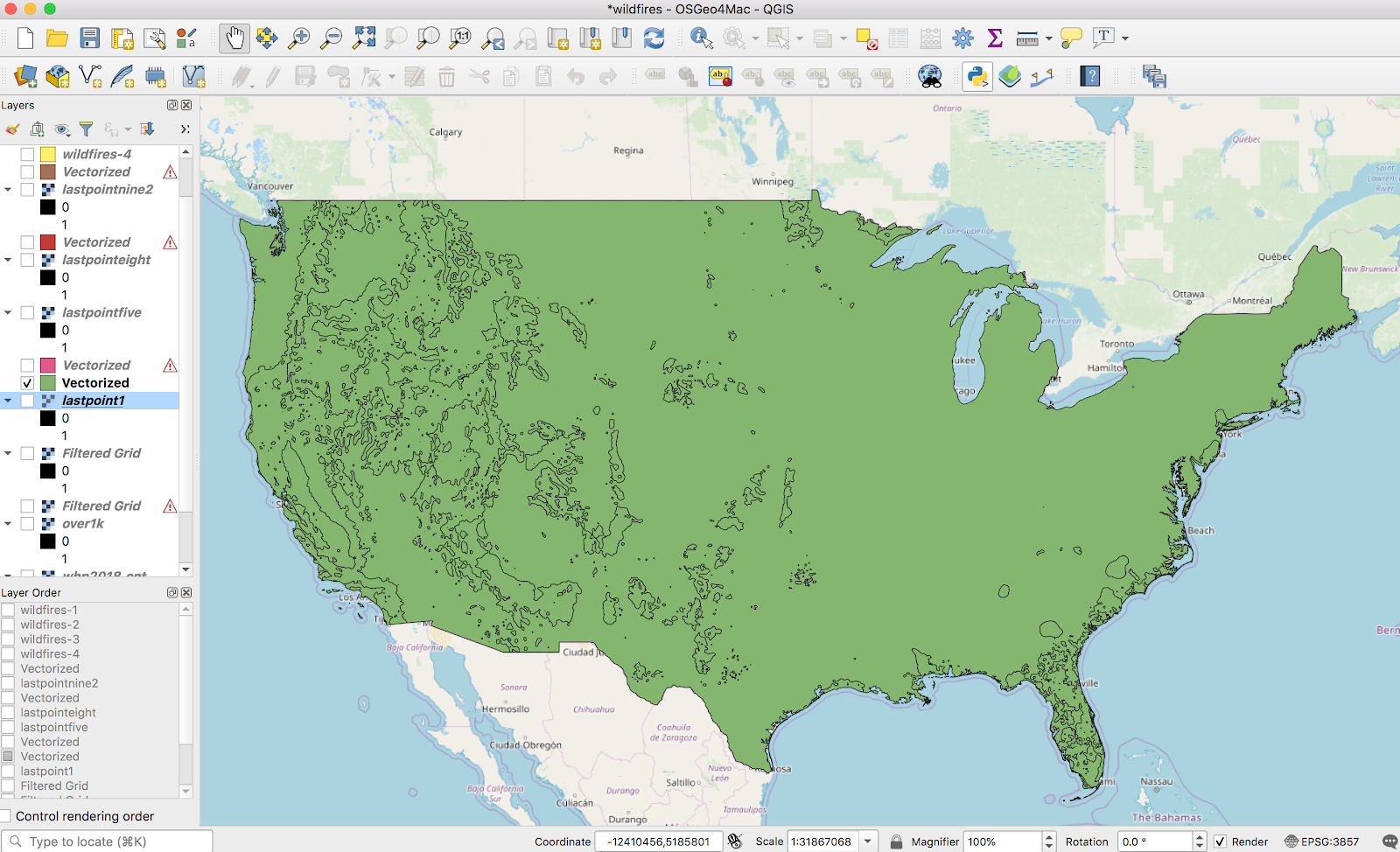
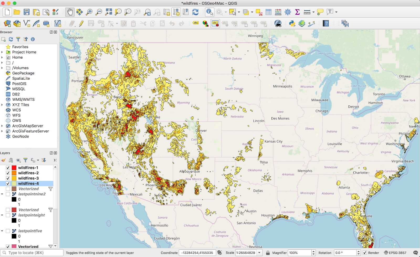
Fast forward a bit, filtering out the 0-value shape from the vector layer, rinse-and-repeating with 3 more thresholds, and adding some colors, it looks pretty good:
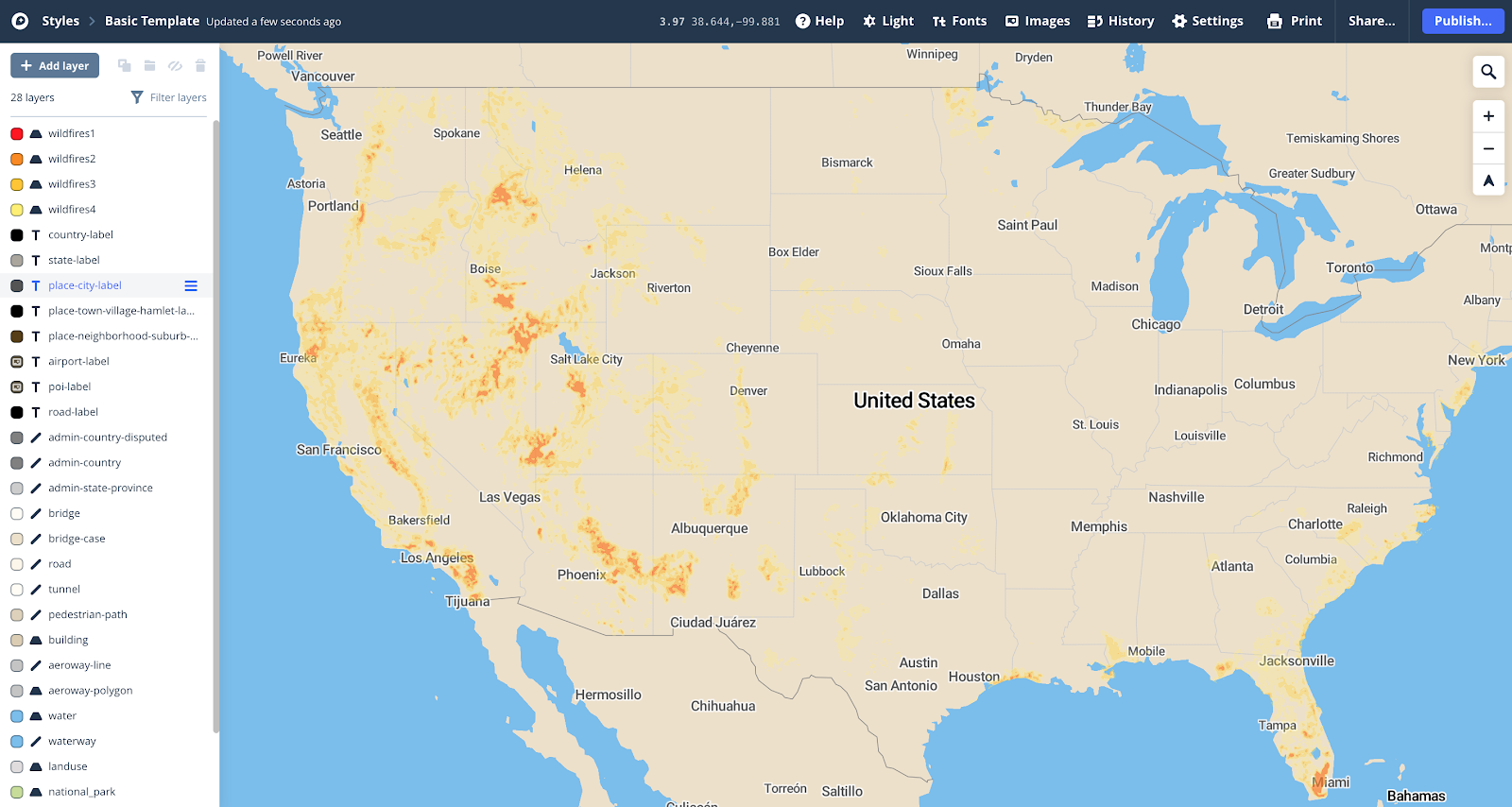
I want this on Mapbox, so I uploaded it there (again, see my older post for how I uploaded this data as an mbtiles file). Applied the same color scheme in a Style there, and it looks nice:
Just as a summary of the before and after, here is Los Angeles with my best attempt at styling the raw raster data:
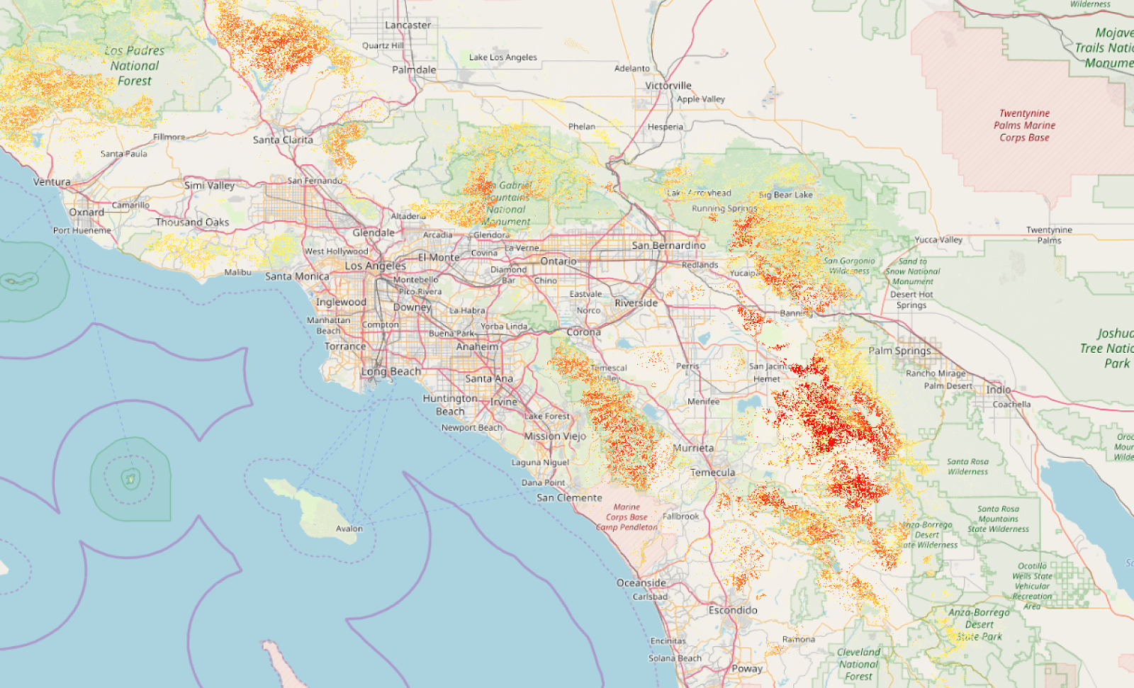
You get the general idea, but it’s not really fun when you zoom in. Here’s it is after the Gaussian filter and banding:
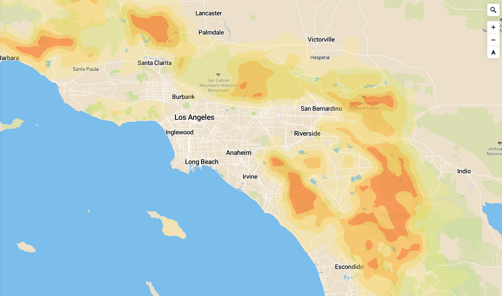
I found these layers a lot easier to work with, and a lot more informative to the end user. It’s now visible as a layer on bunker.land.
I thought this tool was nifty, so hopefully this helps someone else who needs to smooth out some input rasters.

One thought on “Using the QGIS Gaussian Filter on Wildfire Risk Data”